If you’ve started learning programming or computer science, you’ve probably come across the term Big O. At first glance, it may seem like a complex mathematical concept, but it is actually one of the most practical tools for understanding how efficiently algorithms perform.
Big O notation helps developers estimate how an algorithm behaves as the amount of data grows. Instead of measuring execution time in seconds, it focuses on the relationship between input size and performance. This makes Big O useful regardless of programming language, hardware, or operating system.
What Is Big O?
Big O is a mathematical notation used to describe the performance or complexity of an algorithm. Specifically, it explains how the running time or memory usage changes as the input size grows.
Instead of asking, “How many seconds does this algorithm take?” Big O asks:
“How does performance change when the amount of data becomes much larger?”
For example, an algorithm that works well with 100 items may become extremely slow with one million items. Big O helps predict this behavior before software reaches production.
Why Is Big O Important?
Modern applications often process thousands or even millions of records. Choosing an efficient algorithm can dramatically improve speed and reduce resource consumption.
Big O helps developers:
- Compare different algorithms
- Write scalable software
- Reduce processing time
- Improve application performance
- Prepare for technical interviews
- Design efficient systems
Whether you’re building a website, mobile app, database engine, or search platform, understanding algorithm complexity is essential.
Understanding Time Complexity
Time complexity describes how the execution time changes as the input grows.
Imagine searching for a person’s name.
If you search one record at a time, performance depends on the list size.
If the list doubles, the search may also take nearly twice as long.
Different algorithms grow at different rates.
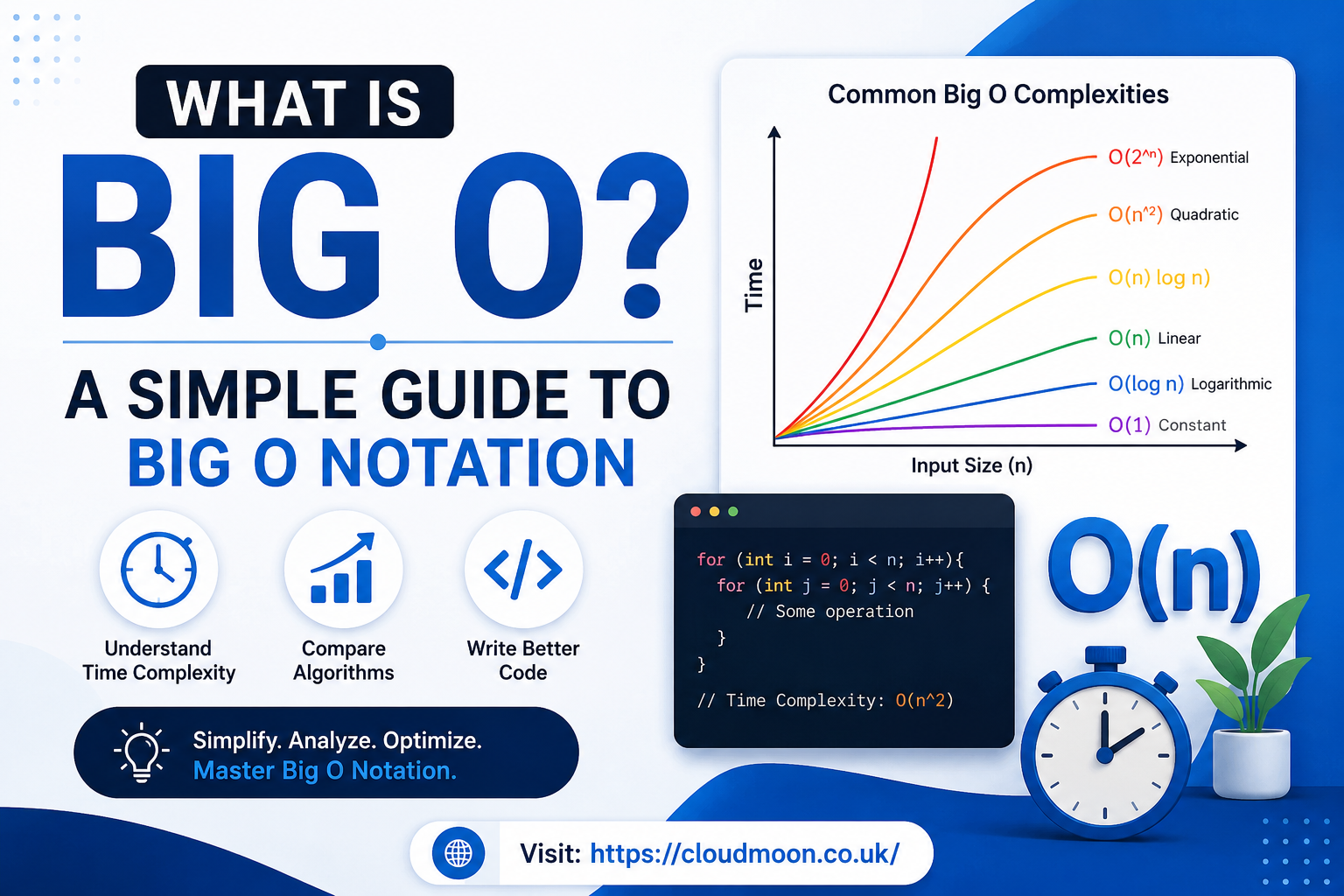
Common Big O Time Complexities
| Big O | Name | Performance |
|---|---|---|
| O(1) | Constant Time | Excellent |
| O(log n) | Logarithmic Time | Very Fast |
| O(n) | Linear Time | Good |
| O(n log n) | Linearithmic Time | Efficient |
| O(n²) | Quadratic Time | Slow for large datasets |
| O(2ⁿ) | Exponential Time | Very Slow |
| O(n!) | Factorial Time | Extremely Slow |
As complexity increases, algorithms become less practical for large amounts of data.
O(1): Constant Time
Constant time means execution remains the same regardless of input size.
Example:
Accessing an element in an array by index.
numbers[5]Whether the array contains 10 items or 10 million, accessing index 5 takes essentially the same amount of work.
This is one of the most efficient complexities.
O(log n): Logarithmic Time
Logarithmic algorithms reduce the search space with each step.
The classic example is binary search.
Instead of checking every value, binary search repeatedly divides the data in half.
Example:
Searching a sorted phone book.
Each comparison eliminates half the remaining possibilities.
This makes logarithmic algorithms extremely efficient for large datasets.
O(n): Linear Time
Linear time means every element must be processed once.
Example:
Finding the maximum number in a list.
For each number
    Compare with current maximum
If there are twice as many elements, the work roughly doubles.
O(n log n): Linearithmic Time
Many efficient sorting algorithms have this complexity.
Examples include:
- Merge Sort
- Heap Sort
- Efficient versions of Quick Sort
These algorithms remain practical even for very large datasets.
O(n²): Quadratic Time
Quadratic complexity often appears with nested loops.
Example:
Comparing every student with every other student.
For each student
    Compare against every student
If the number of students doubles, the number of comparisons grows much faster.
Quadratic algorithms become inefficient with large datasets.
Exponential and Factorial Complexity
Some algorithms grow extremely quickly.
Examples include:
- Solving complex puzzles
- Brute-force password attempts
- Certain recursive problems
As input grows, execution time can become impractical.
Developers generally avoid these algorithms unless absolutely necessary.
Understanding Space Complexity
Big O also measures memory usage.
This is called space complexity.
Some algorithms run quickly but consume a large amount of memory.
Others use very little memory but take longer to execute.
Finding the right balance depends on the application.
Example considerations:
- Mobile devices often prioritize low memory usage.
- High-performance servers may trade memory for speed.
- Embedded systems usually have strict memory limits.
Real-World Examples of Big O
Example 1: Searching a List
Suppose you have a list of 1,000 names.
A simple search checks each name individually.
Complexity:
O(n)
A binary search on a sorted list performs much better.
Complexity:
O(log n)
Example 2: Sorting Data
Suppose an online store sorts products by price.
Using Bubble Sort:
O(n²)
Using Merge Sort:
O(n log n)
For thousands of products, the difference becomes significant.
Example 3: Social Networks
Imagine suggesting friends.
Comparing every user with every other user may result in quadratic complexity.
Efficient indexing and graph algorithms help reduce processing time.
Big O Cheat Sheet
| Operation | Typical Complexity |
| Array Access | O(1) |
| Linear Search | O(n) |
| Binary Search | O(log n) |
| Bubble Sort | O(n²) |
| Merge Sort | O(n log n) |
| Quick Sort (Average) | O(n log n) |
| Hash Table Lookup (Average) | O(1) |
Best, Average, and Worst Cases
Many algorithms behave differently depending on the input.
Best Case
The algorithm finishes quickly.
Example:
Finding an item at the beginning of a list.
Average Case
The most common real-world scenario.
This often provides the most useful performance estimate.
Worst Case
The slowest possible situation.
Developers frequently analyze worst-case complexity to ensure software remains reliable under heavy workloads.
Big O vs Big Omega vs Big Theta
These three notations describe algorithm performance differently.
| Notation | Meaning |
| Big O | Upper performance limit |
| Big Omega (Ω) | Lower performance limit |
| Big Theta (Θ) | Exact growth rate |
Big O is the most widely used because it provides a practical upper bound on how an algorithm scales.
Common Mistakes Beginners Make
When learning Big O, many developers make similar mistakes.
These include:
- Confusing execution time with Big O.
- Ignoring space complexity.
- Assuming every nested loop means O(n²).
- Optimizing too early without identifying bottlenecks.
- Comparing algorithms without considering input size.
Understanding the context is just as important as knowing the notation.
Tips for Improving Algorithm Efficiency
To write more efficient code:
- Choose appropriate data structures.
- Avoid unnecessary loops.
- Use hash tables for fast lookups when suitable.
- Sort data only when needed.
- Cache repeated calculations.
- Measure performance before optimizing.
- Focus on readability alongside efficiency.
Optimization should improve performance without making code difficult to maintain.
When Should You Care About Big O?
Not every project requires deep optimization.
For small scripts handling tiny datasets, readability often matters more than complexity.
However, Big O becomes increasingly important when:
- Building APIs
- Processing large databases
- Creating search engines
- Developing games
- Working with machine learning datasets
- Designing scalable web applications
- Preparing for software engineering interviews
Knowing Big O helps developers make informed decisions before performance problems arise.
Frequently Asked Questions
1. What does Big O measure?
Big O measures how an algorithm’s running time or memory usage grows as the input size increases.
2. Why is Big O important?
It helps developers compare algorithms, write scalable applications, and predict performance with large datasets.
3. Is Big O only used in programming interviews?
No. While it’s common in interviews, Big O is widely used in software development, database design, system architecture, and performance optimization.
4. What is the fastest Big O complexity?
O(1), or constant time, is generally considered the most efficient because performance remains the same regardless of input size.
5. What is the difference between time complexity and space complexity?
Time complexity measures execution speed, while space complexity measures memory usage.
6. Can one algorithm have multiple Big O values?
Yes. An algorithm may have different best-case, average-case, and worst-case complexities depending on the input.
7. Should beginners learn Big O early?
Yes. Learning Big O early builds a strong foundation for writing efficient code and understanding algorithm design.
Conclusion
Understanding Big O is one of the most valuable skills for any programmer. It provides a standardized way to evaluate algorithms, compare solutions, and build software that performs well as data grows. Rather than focusing on exact execution times, Big O highlights how algorithms scale, making it easier to choose the right approach for a given problem.
Whether you’re learning programming, preparing for coding interviews, or developing large-scale applications, mastering Big O notation will help you write more efficient, maintainable, and scalable code. By combining efficient algorithms with appropriate data structures and thoughtful design, you can create software that performs reliably today and continues to perform well as your projects grow.